3
Querying Spatial Data

This chapter describes how the structures of a Spatial Cartridge layer are used to resolve spatial queries and spatial joins. For the sake of clarity, the examples assume that all of the tiles covering all of the elements in a layer are the same size, although this is not required by Spatial Cartridge.

3.1 Query Model

Spatial Cartridge uses a "two-tier" query model to resolve spatial queries and spatial joins. The term is used to indicate that two distinct operations are performed in order to resolve queries. The output of both operations yield the exact result set.

The two operations are referred to as primary and secondary filter operations.

The primary filter permits fast selection of a small number of candidate records to pass along to the secondary filter. The primary filter uses approximations in order to reduce computational complexity and is considered a lower cost filter.
The secondary filter applies exact computational geometry to the result set of the primary filter. These exact computations yield the final answer to a query.The secondary filter operations are computationally more expensive, but they are only applied to the relatively small result set from the primary filter.

Figure 3-1 illustrates the relationship between the primary and secondary filters:

Figure 3-1 Query Model

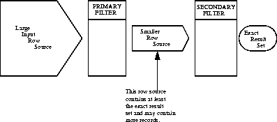
Spatial Cartridge uses a spatial index to implement the primary filter. This is described in detail in following sections.

A function used as a secondary filter is SDO_GEOM.RELATE(), which determines the spatial relationship between two given geometries, such as whether they touch, overlap, or if one is inside the other.

Spatial Cartridge does not require the use of both the primary and secondary filters. In some cases, just using the primary filter is sufficient. For example, the zoom feature in a mapping application queries for data that overlaps a rectangle representing visible boundaries. The primary filter very quickly returns a superset of the query. The mapping application can then apply clipping routines to display the target area.

3.2 Spatial Data Model

An important concept in the spatial data model is that each element is represented in the <layername>_SDOINDEX table by a set of exclusive and exhaustive tiles. This means that the tiles fully cover the object (exhaustive) and that no tiles overlap each other (exclusive).

Consider the following layer containing several objects in Figure 3-2. Each object is labeled with its SDO_GID. The relevant cover tiles are labeled with `Tn'.

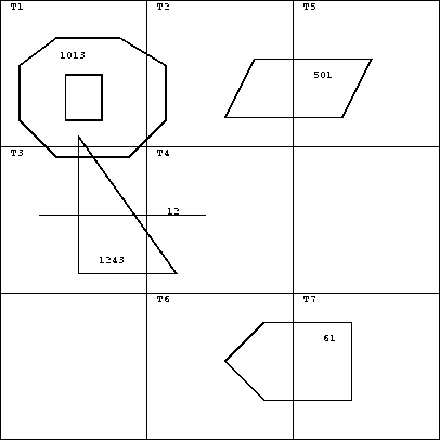
Figure 3-2 Tessellated Layer with Multiple Objects

The Spatial Cartridge layer tables would have the following information stored in them for these geometries as shown in Table 3-1, Table 3-2, and Table 3-3:

SDO_ORDCNT (NUMBER)
4

SDO_GID (NUMBER)	SDO_ESEQ (NUMBER)	SDO_ETYPE (NUMBER)	SDO_SEQ (NUMBER)	SDO_X1 (NUMBER)	SDO_Y1 (NUMBER)	SDO_X2 (NUMBER)	SDO_Y2 (NUMBER)
1013	0	3	0	P1(X)	P1(Y)	P2(X)	P2(Y)
1013	0	3	1	P2(X)	P2(Y)	P3(X)	P3(Y)
1013	0	3	2	P3(X)	P3(X)	P4(X)	P4(Y)
1013	0	3	3	P4(X)	P4(Y)	P5(X)	P5(Y)
1013	0	3	4	P5(X)	P5(Y)	P6(X)	P6(Y)
1013	0	3	5	P6(X)	P6(Y)	P7(X)	P7(Y)
1013	0	3	6	P7(X)	P7(Y)	P8(X)	P8(Y)
1013	0	3	7	P8(X)	P8(Y)	P1(X)	P1(Y)
1013	1	3	0	G1(X)	G1(Y)	G2(X)	G2(Y)
1013	1	3	1	G2(X)	G2(Y)	G3(X)	G3(Y)
1013	1	3	2	G3(X)	G3(Y)	G4(X)	G4(Y)
1013	1	3	3	G4(X)	G4(Y)	G1(X)	G1(Y)
501	0	3	0	A1(X)	A1(Y)	A2(X)	A2(Y)
501	0	3	1	A2(X)	A2(Y)	A3(X)	A3(Y)
501	0	3	2	A3(X)	A3(Y)	A4(X)	A4(Y)
501	0	3	3	A4(X)	A4(Y)	A1(X)	A1(Y)
1243	0	3	0	B1(X)	B1(Y)	B2(X)	B2(Y)
1243	0	3	1	B2(Y)	B2(Y)	B3(X)	B3(Y)
1243	0	3	2	B3(X)	B3(Y)	B1(X)	B1(Y)
12	0	2	0	D1(X)	D1(Y)	D2(X)	D2(Y)
61	0	3	0	C1(X)	C1(Y)	C2(X)	C2(Y)
61	0	3	1	C2(X)	C2(Y)	C3(X)	C3(Y)
61	0	3	2	C3(X)	C3(Y)	C4(X)	C4(Y)
61	0	3	3	C4(X)	C4(Y)	C5(X)	C5(Y)
61	0	3	4	C5(X)	C5(Y)	C1(X)	C1(Y)

SDO_GID (NUMBER)	SDO_CODE (RAW)
`1013`	T1
1013	T2
1013	T3
501	T2
501	T5
1243	T2
1243	T3
1243	T4
12	T3
12	T4
61	T6
61	T7

Table 3-1 <layername>_SDOLAYER

SDO_ORDCNT (NUMBER)

4

Table 3-2 <layername>_SDOGEOM

SDO_GID (NUMBER) SDO_ESEQ (NUMBER) SDO_ETYPE (NUMBER) SDO_SEQ (NUMBER) SDO_X1 (NUMBER) SDO_Y1 (NUMBER) SDO_X2 (NUMBER) SDO_Y2 (NUMBER)

1013

0

3

0

P1(X)

P1(Y)

P2(X)

P2(Y)

1013

0

3

1

P2(X)

P2(Y)

P3(X)

P3(Y)

1013

0

3

2

P3(X)

P3(X)

P4(X)

P4(Y)

1013

0

3

3

P4(X)

P4(Y)

P5(X)

P5(Y)

1013

0

3

4

P5(X)

P5(Y)

P6(X)

P6(Y)

1013

0

3

5

P6(X)

P6(Y)

P7(X)

P7(Y)

1013

0

3

6

P7(X)

P7(Y)

P8(X)

P8(Y)

1013

0

3

7

P8(X)

P8(Y)

P1(X)

P1(Y)

1013

1

3

0

G1(X)

G1(Y)

G2(X)

G2(Y)

1013

1

3

1

G2(X)

G2(Y)

G3(X)

G3(Y)

1013

1

3

2

G3(X)

G3(Y)

G4(X)

G4(Y)

1013

1

3

3

G4(X)

G4(Y)

G1(X)

G1(Y)

501

0

3

0

A1(X)

A1(Y)

A2(X)

A2(Y)

501

0

3

1

A2(X)

A2(Y)

A3(X)

A3(Y)

501

0

3

2

A3(X)

A3(Y)

A4(X)

A4(Y)

501

0

3

3

A4(X)

A4(Y)

A1(X)

A1(Y)

1243

0

3

0

B1(X)

B1(Y)

B2(X)

B2(Y)

1243

0

3

1

B2(Y)

B2(Y)

B3(X)

B3(Y)

1243

0

3

2

B3(X)

B3(Y)

B1(X)

B1(Y)

12

0

2

0

D1(X)

D1(Y)

D2(X)

D2(Y)

61

0

3

0

C1(X)

C1(Y)

C2(X)

C2(Y)

61

0

3

1

C2(X)

C2(Y)

C3(X)

C3(Y)

61

0

3

2

C3(X)

C3(Y)

C4(X)

C4(Y)

61

0

3

3

C4(X)

C4(Y)

C5(X)

C5(Y)

61

0

3

4

C5(X)

C5(Y)

C1(X)

C1(Y)

Table 3-3 <layername>_SDOINDEX

SDO_GID (NUMBER) SDO_CODE (RAW)

1013

T1

1013

T2

1013

T3

501

T2

501

T5

1243

T2

1243

T3

1243

T4

12

T3

12

T4

61

T6

61

T7

3.3 Spatial Query

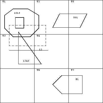
A typical spatial query is to request all objects that lie within a defined fence or window. A query window is defined in Figure 3-3 by the dotted line box. A dynamic query window refers to a fence that is not defined in the database, but that must be defined and indexed prior to using it.

Figure 3-3 Tessellated Layer with a Query Fence

3.3.1 Dynamic Query Window

If a query window does not already exist in the database, you must first insert it and create and index for it. Because not all Oracle users may have insert privileges, Spatial Cartridge includes the SDO_WINDOW PL*SQL package. See Chapter 7, "Window Functions"for more information.

The SDO_WINDOW package is not automatically installed when you install Spatial Cartridge. This allows a DBA to control the schema under which this package operates. Choose an Oracle user that has insert privilege and compile the SDO_WINDOW package under that user. For example, you could choose the mdsys Oracle user:

sqlplus mdsys/password

SQL> @$ORACLE_HOME/md/admin/sdowin.sql 
SQL> @$ORACLE_HOME/md/admin/prvtwin.plb

After compiling, the routines are available for use. When you call a routine in this package, and the routine performs an INSERT operation, the insert will occur under the mdsys schema. Note that it is not a requirement to use the mdsys account. You can select any Oracle user with insert privileges.

If you need to perform other INSERT, UPDATE, or DELETE operations, and you cannot guarantee that the user of your application has those privileges, you can write your own PL*SQL package similar to the SDO_WINDOW package. You will have to compile your package under a user with the required database privileges.

3.3.2 Primary Filter

To resolve the window query shown in Figure 3-3, build a layer for the query fence if it is not already defined:

SQL> EXECUTE MDSYS.SDO_WINDOW.CREATE_WINDOW_LAYER (fencelayer, DIMNUM1, LB1, 
UB1, TOLERANCE1, DIMNAME1, DIMNUM2, LB2, UB2, TOLERANCE2, DIMNAME2)

Next, insert the ordinates for the query fence into the layer tables:

SQL> EXECUTE DBMS_OUTPUT.PUTLINE(TO_CHAR(MDSYS.SDO_WINDOW.BUILD_WINDOW_FIXED 
(comp_user, fencelayer, SDO_ETYPE, TILE_SIZE, X1, Y1, X2, Y2, X3, Y3, X4, Y4, 
X1, Y1)));

Query SDO_LEVEL from the <fencelayer>_SDOLAYER table to pass the correct TILE_SIZE to SDO_WINDOW.BUILD_WINDOW_FIXED.

Now you can construct a query that joins the index of the query window to the appropriate layer index and determines all elements that have these tiles in common. The following SQL query form is used:

SELECT DISTINCT A.SDO_GID, B.SDO_GID

FROM <layer1>_SDOINDEX A, <fencelayer>_SDOINDEX B

WHERE	 		A.SDO_CODE = B.SDO_CODE 
and B.SDO_GID = {GID returned from SDO_WINDOW.BUILD_WINDOW_FIXED};

The result set of this query is the PRIMARY filter set. In this case, the result set is:

 { 1013,501,1243,12 }

3.3.3 Secondary Filter

The SECONDARY filter performs exact geometry calculations of the tiles selected by the PRIMARY filter. The following example shows the first and second pass filters:

SELECT SDO_X1, SDO_Y1, SDO_X2, SDO_Y2, SDO_X3, SDO_Y3, SDO_X4, SDO_Y4
FROM <layer1>_SDOGEOM,
(
SELECT SDO_GID GID1
   FROM (
          SELECT DISTINCT A.SDO_GID
             FROM <layer1>_SDOINDEX A,
                  <fence>_SDOINDEX B
             WHERE A.SDO_CODE = B.SDO_CODE         
         )
   WHERE SDO_GEOM.INTERACT('<layer1>', GID1, '<fence>', 1) = 'TRUE'
   )
WHERE SDO_GID = GID1;

This query would return all the geometry IDs that lie within or overlap the window. In this example, the results of the second pass filter would be:

{1243,1013}

The example in this section uses the SDO_GEOM.INTERACT() secondary filter. Both the INTERACT() and RELATE() secondary filters are overloaded functions. For better performance, use the versions that explicitly list the coordinates of the fence whenever possible. See Chapter 6, "Geometry Functions" for details on using these functions.

3.4 Spatial Join

A spatial join is the same as a regular join except that the predicate involves a spatial operator. In Spatial Cartridge, a spatial join takes place between two layers; specifically, two <layername>_SDOINDEX tables are joined.

Example 3-1

Spatial joins can be used to answer questions such as, "which highways cross national parks?"

This query could be resolved by joining a layer that stores national park geometries with one that stores highway geometries.The following table structures will be used to illustrate how the join would be accomplished for this example: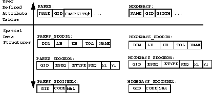

The PRIMARY filter would identify pairs of PARK GIDs and HIGHWAY GIDs that cross in the index. The query that performs the PRIMARY filter join is:

SELECT DISTINCT A.SDO_GID, B.SDO_GID 

FROM PARKS_SDOINDEX A, HIGHWAYS_SDOINDEX B 

WHERE A.SDO_CODE BETWEEN B.SDO_CODE AND B.SDO_MAXCODE

OR B.SDO_CODE BETWEEN A.SDO_CODE AND A.SDO_MAXCODE;

The result set of the PRIMARY filter must be passed through the SECONDARY filter to get the exact set of PARKS/HIGHWAYS GID pairs that cross. The query that performs the SECONDARY filtering is: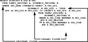

Suppose the original query had asked, "which 4-lane highways cross national parks." You could modify the preceding SQL statement to join back to the HIGHWAYS table where HIGHWAYS.WIDTH=4. This combination of spatial and relational attributes in a single query is one of the primary reasons for using Spatial Cartridge.

3 Querying Spatial Data